Markov chains, memorylessness, and a small calculation in diffusion models
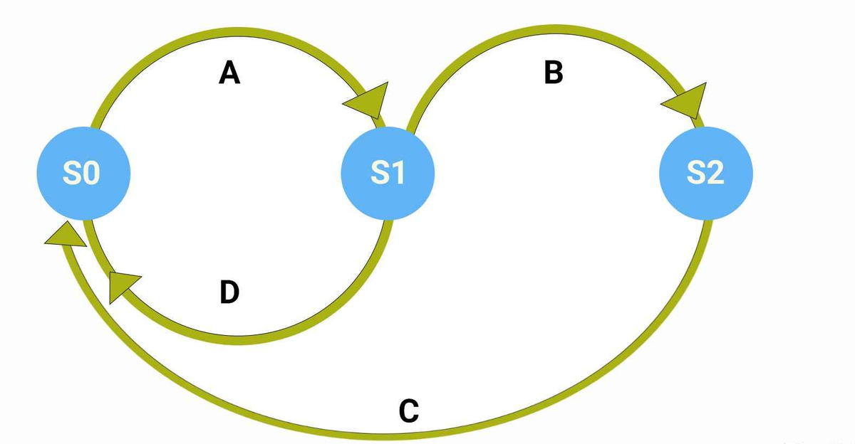
Recently I was working through some calculations involving diffusion models for a computational biology project. It's a nice project, and I hope to have the paper finished soon. It mainly has to do with the dynamics of protein interactions. A key step in the calculation relies on the forward Markov assumption, providing a nice example of how transition matrices, conditional probability, Bayes' rule, and the Markov property fit together.
The biological setting is not especially important for what follows. We can treat the problem simply as a discrete probability calculation. The first thing to know is about the very strong assumption underlying the notion of a Markov chain: if we want to predict the future of a sequence, all that matters is its current state. The states that came before the current state have no additional influence on the future except through their effect on the present. To give some intuition: it is as if, in trying to predict tomorrow's weather, we were allowed to examine today's weather but were not allowed to look at yesterday's weather. Whatever happened yesterday matters only insofar as it has already influenced what the weather is like today.
Mathematically, if we have a sequence of random variables
\[ s_0,s_1,s_2,\ldots,s_t, \]
the Markov property says
\[ q(s_t\mid s_{t-1},s_{t-2},\ldots,s_0) = q(s_t\mid s_{t-1}). \]
This deceptively simple statement does quite a lot of work.
A sequence of probabilistic transitions
Imagine that we have some object that can occupy one of \( K \) discrete states. Let's assume the state is an amino-acid identity at a particular residue position, in which there are \( K = 20 \) possible categories corresponding to the standard amino acids.
At each step of a diffusion process, the identity may be probabilistically corrupted. If the state at step \(t-1 \) is \( i \), it may remain \( i \), or it may change to some other category \( j \). We encode all of these one-step probabilities in a transition matrix \( Q_t \), defined by
\[ [Q_t]_{ij} = q(s_t=j\mid s_{t-1}=i). \]
The important point here is what the subscript \( t \) actually means. The matrix \( Q_t \) describes the particular transition
\[ s_{t-1}\longrightarrow s_t. \]
The chain can thus be drawn explicitly as
\[ s_0 \xrightarrow{Q_1} s_1 \xrightarrow{Q_2} s_2 \xrightarrow{Q_3} \cdots \xrightarrow{Q_t} s_t. \]
So \( Q_1 \) tells us how to go from \( s_0 \) to \( s_1 \), \( Q_2 \) tells us how to go from \(s_1 \) to \( s_2 \), and, in general,
\[ Q_t: s_{t-1}\longrightarrow s_t. \]
Notice the distinction between a one-step transition and a many-step transition. A one-step transition moves a system from its current state to the next immediate state in one step of the process, while a many-step transition tracks the path or probability of reaching a future state over multiple steps. To use the weather example: it is the difference of predicting the weather three days from now, or simply moving from a sunny weather state today to a rainy weather state tomorrow.
From one step to many
Let \( a,b \) be some specific states. Suppose that initially \( s_0 = a \), the initial state. We might then want to ask: what is the probability that after two steps we find \( s_2 = b \)? There is of course an intermediate state \( s_1 \), but we do not know what it is. It might be any of the \( K \) possible categories of the amino acids. So, what we do, is sum over every possible intermediate state \( j \) such that
\[ q(s_2=b\mid s_0=a) = \sum_{j=1}^{K} q(s_2=b\mid s_1=j,s_0=a) q(s_1=j\mid s_0=a). \]
Here the Markov property enters for the first time. Once \( s_1=j \) is known, the value of \( s_0 \) provides no additional information about \( s_2 \). Hence
\[ q(s_2=b\mid s_1=j,s_0=a) = q(s_2=b\mid s_1=j). \]
By definition of our transition matrices,
\[ q(s_1=j\mid s_0=a) = [Q_1]_{aj}, \]
and
\[ q(s_2=b\mid s_1=j) = [Q_2]_{jb}. \]
Therefore
\[ q(s_2=b\mid s_0=a) = \sum_{j=1}^{K} [Q_1]_{aj}[Q_2]_{jb}. \]
But this sum is exactly the definition of matrix multiplication:
\[ [Q_1Q_2]_{ab} = \sum_{j=1}^{K} [Q_1]_{aj}[Q_2]_{jb}. \]
We therefore obtain
\[ q(s_2=b\mid s_0=a) = [Q_1Q_2]_{ab}. \]
This is a particularly nice result. What this tells us is that a product of transition matrices automatically performs the sum over every possible intermediate path. The same argument continues for more steps. Let
\[ \overline Q_t = Q_1Q_2\cdots Q_t. \]
Then, we see,
\[ [\overline Q_t]_{ab} = q(s_t=b\mid s_0=a). \]
The bar notation here distinguishes the accumulated transition \(s_0\longrightarrow s_t \) from the single transition \( s_{t-1}\longrightarrow s_t. \) In short, \( Q_t = \text{one-step transition} \), whereas \( \overline Q_t = \text{all transitions from step} \) \(0\) through step \(t\).
Turning the question around
Now for the calculation I originally wanted to understand. Suppose we know two things \( s_0 = a \) and \( s_t=b \). That is, we know where the process started and where it ended up after \( t \) diffusion steps. We now ask a backward-looking question:
Given that the process started at \( a \) and ended at \( b \), how plausible is it that the immediately preceding state \( s_{t-1} \) was some particular category \( j \)?
Mathematically, this is tantamount to wanting to ascertain
\[ q(s_{t-1} = j\mid s_t=b,s_0=a). \]
Notice, this is a posterior probability, so Bayes' rule is the natural starting point. Indeed, it is not difficult to see that Bayes' rule gives
\[ q(s_{t-1}=j\mid s_t=b,s_0=a) = \frac{ q(s_t=b\mid s_{t-1}=j,s_0=a) q(s_{t-1}=j\mid s_0=a) }{ q(s_t=b\mid s_0=a) }. \]
It is worth pausing here, because each of the three factors has a slightly different meaning. The first asks \( q(s_t=b\mid s_{t-1}=j,s_0=a) \), which is the probability of making the final transition from\( j \) to \( b \). The second asks \( q(s_{t-1}=j\mid s_0=a) \), which is the probability of reaching \( j \) from the initial state \( a \) during the preceding \( t-1 \) steps. Finally, the denominator asks \( q(s_t=b\mid s_0=a) \) is the total probability of reaching \( b \) from \( a \). The whole result becomes transparent once we place these three probabilities on the chain
\[ a = s_0 \xrightarrow{Q_1} s_1 \xrightarrow{Q_2} \cdots \xrightarrow{Q_{t-1}} s_{t-1} = j \xrightarrow{Q_t} s_t = b. \]
The forward Markov assumption
Consider the first factor. The Markov assumption says that once \( s_{t-1} = j \) is known, earlier states no longer provide additional information about the next state. Therefore,
\[ q(s_t=b\mid s_{t-1}=j,s_0=a) = q(s_t=b\mid s_{t-1}=j). \]
And because this is the single transition such that \( s_{t-1}\longrightarrow s_t \), the appropriate transition matrix \( Q_t \) giving
\[ q(s_t=b\mid s_{t-1}=j) = [Q_t]_{jb}. \]
Why \( Q_t \), rather than\( Q_{t-1} \)? Because \( Q_{t-1} \) describes \( s_{t-2}\longrightarrow s_{t-1} \), whereas the probability we are presently calculating concerns \( s_{t-1}\longrightarrow s_t \).
We already know that the system is at \( j \) at time \( t-1 \). We do not need to sum over its previous history. We only need the probability of the final jump \( j\longrightarrow b \).
Now consider the second factor \( q(s_{t-1}=j\mid s_0=a). \) Now we are starting \( s_0=a \) and asking for the probability of reaching \( s_{t-1}=j. \) That journey contains all of the transitions \( Q_1,Q_2,\ldots,Q_{t-1}. \) Consequently,
\[ q(s_{t-1}=j\mid s_0=a) = [Q_1Q_2\cdots Q_{t-1}]_{aj}. \]
Using shorthand,
\[ \overline Q_{t-1} = Q_1Q_2\cdots Q_{t-1}, \]
so that
\[ q(s_{t-1}=j\mid s_0=a) = [\overline Q_{t-1}]_{aj}, \]
in which we have a multi-step probability. Notice also why \( s_0 \) cannot be removed here using the Markov property. We are not conditioning on\( s_{t-2} \) or \( s_{t-1} \) and asking what happens next. We are explicitly asking for the probability of reaching \( j \) given the initial state \( a \).
Finally, for the denominator term, \( q(s_t=b\mid s_0=a) \), asks for the probability of making the complete journey \( s_0=a \longrightarrow s_t=b. \) Every transition from \( Q_1 \) through \( Q_t \) is involved so that we may write
\[ q(s_t=b\mid s_0=a) = [Q_1Q_2\cdots Q_t]_{ab}. \]
Therefore, it is clear we have
\[ q(s_t=b\mid s_0=a) = [\overline Q_t]_{ab}, \]
capturing the accumulated effect of all \( t \) transitions.
Putting everything together
Returning to Bayes' rule, direct substitution gives
\[ q(s_{t-1}=j\mid s_t=b,s_0=a) = \frac{ [Q_t]_{jb} [\overline Q_{t-1}]_{aj} }{ [\overline Q_t]_{ab} }. \]
For the denominator, note that the total probability of reaching \( b \) from \( a \) includes all possible values of the intermediate state \( s_{t-1} \). Indeed,
\[ [\overline Q_t]_{ab} = \sum_{j=1}^{K} [\overline Q_{t-1}]_{aj} [Q_t]_{jb} \]
follows immediately because \( \overline Q_t = \overline Q_{t-1}Q_t. \) So the denominator normalises the different possible values of \( j \).
Altogether, this, really, is Bayes' rule doing exactly what Bayes' rule always does: taking a prior plausibility and updating it in light of some additional information.
The individual ingredients are all elementary, but together they form a nice recipe. There is a Markov chain, a collection of transition matrices, some ordinary matrix multiplication, and Bayes' rule. In combination, they let us answer a rather specific backward question about a stochastic process. The forward Markov assumption tells us that, for that last transition, once \( s_{t-1} \) is known, the history that produced \( s_{t-1} \) is irrelevant to predicting \( s_t \). There is something pleasingly economical about that. A potentially complicated history is compressed into the present state, while matrix multiplication quietly takes care of all the possible paths that could have produced it.
For the diffusion-model calculation that led me here, these \( s_t \) are artificial noisy states rather than physical time evolution. But the probabilistic logic is quite general, and I think the derivation makes for a particularly clean illustration of what the Markov assumption actually buys us in practice.