Measuring the depth of a model: how deep is deep?
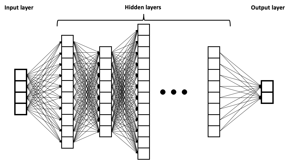
A fascinating question in modern machine learning has to do with how to measure the depth of a model. In the simplest setting, neural networks are either recurrent or feedforward. A feedforward network contains no directed cycles in its computational graph, which means it can be neatly organised into successive layers. Conventionally, when a network contains many of these layers, it is considered deep.
But where exactly does "shallow" end and "deep" begin? Is there some principled number of layers beyond which a shallow neural network becomes a deep neural network? If we consider the somewhat dated premise that simply stacking more layers guarantees better performance, another question follows: why should having more layers help? Over the last decade, answers to these questions have changed considerably.
Naively, one might imagine that there exists some universal numerical threshold \(L^\star \), almost like a phase transition, at which a neural network suddenly becomes deep
\[ \text{shallow} \quad\overset{L=L^\star}{\longrightarrow}\quad \text{deep}.\]
But the modern view suggests there is no such threshold. Instead, a growing body of rigorous research indicates that searching for one is asking the wrong question. This is because, although the traditional view of depth in terms of counting layers in a feedforward network has not disappeared, it has proved insufficient. Residual networks, recurrent and weight-tied architectures, transformers, neural ordinary differential equations, and implicit models, have each progressively separated several concepts that once coincided: the number of parameterised layers, the number of sequential computational steps, the lengths of paths through a network, and the depth of the representations or concepts learned by that network. The science has thus led to a rather different conception of depth: it would seem better viewed as a computational resource than as a categorical property separating one kind of neural network from another.
The classical picture: depth as a hierarchy of representations
To ground this discussion mathematically, and in terms of a quantifiable picture, let's first consider the classical view. It is perhaps best summarised in the authoritative textbook Deep Learning by Goodfellow, Bengio and Courville. They first approach the notion of deep learning through representation learning and composition. The idea is very simple: deep networks may be viewed hierarchically such that a complex concept can be represented in terms of simpler concepts, which are themselves represented in terms of still simpler ones. In the canonical computer-vision example,
\[ \text{pixels} \rightarrow \text{edges} \rightarrow \text{corners and contours} \rightarrow \text{object parts} \rightarrow \text{objects}. \]
In this view, a simple feedforward network naturally expresses the idea that instead of learning a single mapping
\[ y=f(x), \]
it computes \( h_1=f_1(x), \) \( h_2=f_2(h_1), \) and eventually
\( y=f_L(h_{L-1}) \) so that
\[ f=f_L \circ f_{L-1} \circ \cdots \circ f_1. \]
Each layer supplies a new representation on which the next layer operates.
This intuitive perspective partly explains why the word deep became so natural in its usage: it suggested a hierarchy of abstractions analogous, at least very loosely, to hierarchical processing in biological sensory systems. But as Goodfellow, Bengio, and Courville also discuss, there is also a second interpretation that, arguably, has proved even more important in the last decade. Rather than interpreting a layer as a humanised concept, the network can be regarded as executing a multi-step computer program. Each layer then represents another sequential transformation of an internal state, nothing more. As depth increases correlative to the number of layers, later operations make use of intermediate results computed by earlier operations. Thus, one may write schematically
\[ h_0\rightarrow h_1\rightarrow h_2\rightarrow\cdots\rightarrow h_L, \]
which, it should be noted, is not necessarily representative of a progression from edges to objects. This chain may instead be thought of as a sequence of computational states.
Comparatively, the distinction between depth as representation hierarchy and depth as sequential computation has become increasingly important.
A classical puzzle: if one hidden layer is universal, why should depth matter?
There was, however, an apparent mathematical objection to the whole deep-learning programme. In an intuitive framing, the view was that having several layers or one layer was equivalent in terms of the actual functions represented by a neural network. This came in the form of the universal approximation theorem. Universal approximation created an apparent puzzle, not because shallow and deep finite networks necessarily represent identical function classes; rather, classical results showed that networks with only a single hidden layer are already dense in broad target function spaces under suitable approximation criteria (see also Prince's textbook for insightful discussion). Depth therefore does not appear necessary merely to obtain universality.
An important early form of universal approximation was proved by Cybenko in 1989. The theorem states a family of neural network functions is a dense set within a larger space of functions they are intended to approximate. That is, for any function \(f \) from a given function space, there exists a sequence of neural networks \(\phi_1, \phi_2, \dots \) from the family, such that \( \phi_n \rightarrow f \) according to some criterion. A later, more general characterisation due to Leshno, Lin, Pinkus and Schocken (1993) established the importance of non-polynomial activation functions. A convenient vector-valued formulation proceeds along the following lines:
Let \( C(X,\mathbb{R}^m)\) denote the set of continuous functions from a subset \(X\) of a Euclidean \(\mathbb{R}^n\) space to a Euclidean space \(\mathbb{R}^m\). Let \(\sigma \in C(\mathbb{R},\mathbb{R})\). Note that \((\sigma \circ x)_i = \sigma(x_i)\), so \(\sigma \circ x \) denotes \( \sigma\) applied to each component of \(x\).
Then \(\sigma\) is not polynomial iff for every \( n \in \mathbb{N}, m \in \mathbb{N}\), compact \(K \subseteq \mathbb{R}^n\), \(f \in C(K,\mathbb{R}^m)\), \(\varepsilon > 0\) there exist \(k \in \mathbb{N}\), \(A \in \mathbb{R}^{k \times n}\), \(b \in \mathbb{R}^k\), \(C \in \mathbb{R}^{m \times k}\) such that
\[ \sup_{x \in K} \| f(x)-g(x) \| < \varepsilon \]
where \(g(x) = C \cdot (\sigma \circ (A \cdot x + b)).\)
Classical universal approximation results showed that feedforward networks containing only a single hidden layer can approximate extremely broad classes of functions arbitrarily closely, provided the hidden layer is sufficiently wide. The results of Hornik, Stinchcombe and White are among the classic statements of this fact. Schematically,
\[ \forall \epsilon>0, \quad \exists\,N_{\text{shallow}} \quad\text{such that} \quad \| N_{\text{shallow}}-f \| <\epsilon . \]
Hence, the classically defined question of great interest emerged: if shallow networks can already approximate essentially any function of interest, what exactly does depth add? In fact, this question featured prominently as late as the early and mid-2010s, including the Cross Validated discussion that motivated this post. It is also explicitly addressed in Goodfellow et al.'s textbook.
It turns out, not least thanks to modern approximation and representation theory, that a more rigorous picture may be framed in terms of the following resolution: universal approximation is a statement about existence, not efficiency. The resolution, as I have learned it, is now fundamental to modern approximation theory. It suggests that a shallow network may be capable of representing a function while requiring an enormous number of hidden units to do so.
Consequently, the interesting quantity is not simply whether a network can approximate \(f \), but the resources needed to approximate it. Schematically, for a specified architecture or computational model \( \mathcal{A} \), one may write
\[ C_{L,\mathcal{A}, \mathcal{X}}(f,\varepsilon) := \]
\[ \inf \{\text{cost}(N): N \in\mathcal{N}_{\mathcal{A}}, D_{\mathcal{A}}(N) \leq L, \| N - f \|_{\mathcal{X}} \leq \varepsilon \}, \]
which, schematically, describes the resource trade-off with individual depth-separation theorems. Here \(\mathcal{A}\) specifies the architecture, activation functions, or allowed computational primitives, \( \| \cdot \|_{\mathcal{X}} \) specifies the approximation criterion, and \( \text{cost}(N) \) denotes the particular resource being measured. Depending on the theorem, this might be width, number of units, number of parameters, or another explicitly specified complexity measure. These resources are not interchangeable, so the chosen notion of cost is part of the statement being studied. The question then becomes whether
\[ C_{L-1, \mathcal{A}, \mathcal{X}}(f,\epsilon) \gg C_{L, \mathcal{A},\mathcal{X}}(f,\epsilon), \]
which is the modern depth-separation question. Indeed, by the middle of the 2010s, increasingly strong mathematical results showed that depth can provide dramatic representational advantages. Montúfar, Pascanu, Cho, and Bengio studied piecewise-linear networks and showed how successive layers can create large numbers of linear regions. The important idea is not merely that a deep ReLU network contains many pieces, but that composition allows pieces of computation to be repeatedly reused across layers.
Two particularly influential results followed in 2016: i) Eldan and Shamir exhibited a relatively simple function representable by a small three-layer network that cannot be approximated to comparable accuracy by a two-layer network unless the shallower network has width exponential in the input dimension. As Eldan and Shamir count the output layer, their depth-two network has one hidden layer and their depth-three network has two hidden layers. ii) Telgarsky then established broader depth hierarchies: functions efficiently represented by networks of substantial depth can require exponentially larger networks if the allowed depth is significantly reduced.
This fundamentally changed the universal-approximation discussion. It established that shallow universal approximation does not imply shallow efficient approximation. More specifically, depth-separation theorems typically concern families of target functions indexed by some growing complexity parameter. In dimension-based separations such as Eldan–Shamir, this parameter is the input dimension \( d \). So, for suitable families \(f_d \), one can obtain behaviour of the schematic form
\[ C_{\text{shallow}}(f_d,\epsilon_0) \geq \exp(cd), \]
while
\[ C_{\text{deep}}(f_d,\epsilon_0) \leq d^q \]
for constants \( c,q >0 \), under the model and approximation criterion of the theorem. This echoes the modern textbook view of depth efficiency in a resource bound sense, namely that functions may require exponentially more shallow units for comparable approximation.
Work on compositional function classes provided another route to essentially the same conclusion. If the target itself possesses a hierarchical structure consisting of low-dimensional constituent functions, a network whose architecture reflects that composition can avoid forms of the curse of dimensionality suffered by an unstructured shallow approximation (see here and here).
This gives mathematical substance to part of the original hierarchical intuition. A deep architecture is particularly natural when the target function itself is compositionally structured. The theory has continued to sharpen. In 2025, Safran, Reichman, and Valiant proved an exponential separation between depth-two and depth-three neural networks for an \(O(1) \)-Lipschitz target, while simultaneously keeping the required approximation accuracy and the scale of the approximation domain constant in dimension, under an exponential bound on the weights of the depth-two competitor. This removed some of the pathologies present in earlier lower-bound constructions, where accuracy requirements or target complexity could deteriorate with dimension.
Thus, there really can be mathematically sharp transitions as depth is increased. But these are not universal transitions between “shallow” and “deep”, as one might understandably intuit to be the case - again, much akin to a phase transition. Instead, they are quantifiable statements of the form
\[ \text{for this function class, under these primitives and resource constraints,} \]
\[ \text{depth }L \text{ is dramatically more efficient than depth }L-1. \]
Put simply, the location of the transition belongs to the problem, not to neural networks in general.
So what is depth, and can it be made rigorous?
There are a few complementary perspectives which, when combined, lead to a more rigorous notion of depth. The first comes from the context of an ordinary multilayer perceptron, in which counting layers works reasonably well because several notions of depth coincide. For example,
\[ h_{\ell+1}=\sigma(W_{\ell} h_{\ell}+b_{\ell}). \]
gives a simple chain of sequential dependencies, so architectural depth, computational depth, and the number of successive representations coincide up to ordinary layer-counting conventions.
The more general mathematical definition is closer to the one used in circuit complexity: depth is the length of the longest sequential dependency chain in a computational graph. For a finite directed acyclic computational graph \(G\), or for a recurrent computation after unrolling it to a fixed horizon, one may write, as aligned with Goodfellow et al.,
\[ D(G)=\max_{p:\,\text{input}\rightsquigarrow\text{output}}\mid p \mid,\]
with \( \mid p \mid \) denoting the number of computational stages along the path, up to the usual edge-versus-vertex counting convention.
But even this definition requires us to specify what counts as an elementary operation. Should a matrix multiplication count as one operation? An attention layer? A scalar multiply-add? A complete convolution? The ambiguity means that the rigorous quantity is really relative to a chosen set of computational primitives \(\mathcal G \) which we may denote by \(D_{\mathcal G}(G).\)
Goodfellow et al. anticipated exactly this point when they compared the depth of a network to the length of a computer program: the length depends partly on the language in which the program is expressed. There is therefore no contradiction between saying that depth is rigorously definable and saying that depth is relative. In fact, it is more precise to say that it is rigorously defined once the computational model has been specified.
ResNets: when nominal depth stops telling the whole story
Residual networks made the inadequacy of raw layer counting particularly obvious. Instead of computing only \( h_{\ell+1}=F_\ell(h_\ell), \) a residual block computes something of the form \(h_{\ell+1}=h_\ell+F_\ell(h_\ell). \) The identity creates short routes through what is nominally a very deep architecture.
The original ResNet work demonstrated empirically that residual parameterisations made networks with more than one hundred layers substantially easier to optimise than conventional feedforward networks of comparable depth. Veit, Wilber and Belongie subsequently proposed an influential interpretation of ResNets as collections of paths of many different lengths. In their experiments with a 110-layer residual network, much of the gradient arose from paths only roughly 10–34 layers long.
This should not be turned into the claim that a 110-layer ResNet is really a 10-layer network. The ensemble-of-paths interpretation is one useful model of residual computation, not a universal definition of effective depth. In particular, under the longest path definition above, the computational graph still possesses its full maximum depth
\[ D_{\max} (G) = \max_p \mid p \mid.\]
What the residual decomposition introduces is a collection - or distribution - of paths with different lengths, whose contributions to forward propagation and gradients need not be equal. Thus the maximum graph depth and the dynamically important path-length structure are distinct properties.
A network can contain many parameterised transformations while information and gradients make use of computational paths of different lengths. ResNets therefore illustrate not that depth has suddenly become a property of a graph, since it already was, but that a single scalar such as maximum path length may not describe all of the graph structure relevant to learning dynamics.
Transformers, recurrence, and depth as computational time
But this isn't the whole picture. The advent of transformers complicates things.
A standard Transformer has a well-defined stack of blocks and therefore a perfectly meaningful architectural depth. Yet an attention block performs a rich global transformation in a single nominal layer. Comparing one transformer layer with one classical multilayer-perceptron layer therefore tells us relatively little unless the allowed primitive operations are specified.
Other architectures go further by explicitly reusing transformations across depth. The Universal Transformer, for example, applies a recurrent self-attention transformation across computational depth, combining Transformer-style parallel interaction with recurrence. For a repeated transformation \(h_{t+1}=F_\theta(h_t), \) the number of distinct parameter sets may be one while the number of sequential computational steps is \(T \)
\[ N_{\text{distinct block parameter sets}}=1, \qquad D_{\text{unrolled}}\sim T. \]
Notice that the number of distinct learned transformations and the number of sequential applications have separated. This idea reaches its logical extreme in Deep Equilibrium Models. A DEQ seeks a fixed point
\[ z^\star=f_\theta(z^\star,x) \]
rather than explicitly representing a finite stack of layers. It can be interpreted as the equilibrium of an infinitely deep, weight-tied network, while implicit differentiation avoids storing the entire unrolled trajectory.
So what, then, is the “number of layers” of a DEQ? It turns out that this question is not especially useful. One can instead measure root-finding iterations, function evaluations, convergence properties, and sequential computation. In this sense, the idealised unrolled depth may be regarded as infinite, whereas the realised numerical computation uses a finite, tolerance dependent number of solver evaluations.
Continuous depth
Neural ordinary differential equations provide a different limiting picture. A residual update
\[ h_{k+1}=h_k+\Delta t f_\theta(h_k,t_k). \]
suggests, as \(\Delta t \) becomes small, the differential equation of the form
\[ \frac{dh(t)}{dt}=f_\theta(h(t),t). \]
Thus, neural ODEs replace a discrete sequence of hidden layers by a continuous evolution. This idea was explicitly introduced in the context of continuous-depth models by Chen, Rubanova, Bettencourt, and Duvenaud in their 2018 paper. Here the integration interval plays a role analogous to model depth; but actual computational effort also depends on the numerical solver and the number of function evaluations required to achieve a requested accuracy. Indeed, the integration interval itself should not be interpreted as an invariant measure of computational complexity: the same continuous dynamics may admit different time parameterisations, while solver effort depends on the numerical problem and requested tolerance. Again, model depth and the amount of sequential computation are related but viewed as no longer identical. This suggests that the historical term deep actually bundles together several distinct quantities, as alluded at the outset. For a plain multilayer perceptron these are closely related. For a modern architecture they may differ substantially.
As we'll see in a following post, once depth is treated as a resource rather than a label, the second question to open this post becomes substantially clearer. If the most up-to-date scientific view is that there is no single accepted explanation for the success of deep neural networks, what is revealed is how there are several mechanisms known to operate in different regimes. To offer a physics analogy, it is like a difference of energy regimes, and, correlatively, from the view of effective field theory, a difference of renormalisation scales.
To conclude with a minor digression:
For the reader with a physics background, this analogy is not to be dismissed as mere allusion. Several research programmes use ideas from renormalisation and effective field theory to analyse particular neural network regimes. Interestingly, there are formal structural correspondences in certain settings, although these do not amount to a single unified theory of deep learning.
Several strands of modern theory explore formal correspondences between neural networks and renormalisation-group ideas, with the difference that the relevant notion of scale need not coincide with network depth. Such approaches ask whether coarse-graining, universality, relevant and irrelevant perturbations, and scale-dependent effective descriptions can illuminate particular neural-network regimes. Foundational work by Pankaj Mehta and David J. Schwab demonstrated an exact mathematical mapping between the variational renormalisation group and a class of deep-learning architectures based on restricted Boltzmann machines. Separately, Henry W. Lin, Max Tegmark, and David Rolnick investigated related physics-inspired explanations and argued that deep architectures can achieve exponential parameter efficiency over shallow variants when the functions or data-generating processes exhibit structures such as locality, symmetry and hierarchical compositionality.
Related work in statistical and effective-field-theory approaches reinforces a regime-dependent view of neural-network behaviour rather than supplying a single universal explanation for DNN success. Within this effective-theory framework, such regime-dependent behaviour is explored in Daniel A. Roberts and Sho Yaida’s monograph, The Principles of Deep Learning Theory, with contributions by Boris Hanin, which develops an effective-theory treatment of neural networks in which width, depth-to-width ratio, initialisation, and training determine the validity of different approximations and the size of finite-width effects. For instance, infinite-width limits can lead to Gaussian-process or kernel descriptions in which feature evolution is strongly restricted, whereas finite-width corrections permit departures from such lazy or kernel-like behaviour and can support representation learning. The analogy with interacting field theories is useful in some theoretical frameworks, but should not be identified with a universal mechanism such as manifold flattening.
Deep learning may therefore also be viewed, within these particular theoretical programmes, as exhibiting a regime structure governed by distinct mathematical scales and approximations. But I'll save deeper discussion on these points for another time.