We will talk frequently about stochastic processes on this blog. They are fundamental to quantitative finance, and a basic understanding of stochastic calculus will be an important prerequisite for many of the topics considered later.

We start with a basic introduction to discrete-time stochastic processes (for more detail see any standard textbook on probability theory), in which the time variable takes values in the non-negative integers. In a later post, we will turn to continuous-time processes, where time takes values in the non-negative real numbers, as in the case of Brownian motion.

We begin by introducing the fundamental object of probability theory: the probability space, denoted by

\[ (\Omega,\mathcal F,\mathbb P). \]

This three-tuple provides a complete mathematical description of randomness, consisting of a non-empty set \( \Omega \) that defines a sample space (i.e., the set of all possible outcomes of the experiment), a \( \sigma \)-algebra \( \mathcal{F} \) of subsets of \( \Omega \), which defines the event space (i.e., the collection of all events to which a probability can be assigned), and a probability measure \( \mathbb{P} \) on \( (\Omega, \mathcal{F}) \), which assigns a probability to each event in \( \mathcal{F} \).

To build intuition, consider the example of rolling a fair die. For a single roll of a fair die, we have

\[ \Omega = \{1,2,3,4,5,6 \}, \qquad \mathcal F = 2^\Omega, \qquad \mathbb P({\omega}) = \frac{1}{6} \quad \text{for each } \omega \in \Omega. \]

Here, \( 2^\Omega \) denotes the set of all subsets of \( \Omega \), meaning every possible event is measurable. To move toward stochastic processes, we consider repeated experiments. Passing from one die roll to an infinite sequence of rolls changes the sample space from \( \{1,…,6} \) to the Cartesian product

\[ \Omega = \{1,2,3,4,5,6 \}^{\mathbb N}. \]

This space is uncountable, and the standard probability model is not defined on its full power set \( 2^{\Omega} \). Instead, we use the product \( \sigma \)-algebra generated by cylinder events, which specify the outcomes of only finitely many coordinate rolls. The probability measure is then chosen so that the coordinate rolls are independent and uniformly distributed. (Further details on this construction can be found in standard textbooks on probability theory).

An element \( \omega \in \Omega \) is now an infinite sequence

\[ \omega = (\omega_1, \omega_2, \omega_3, \dots), \]

where \( \omega_t \) represents the outcome of the die at time \( t \). In this setting, a single \( \omega \) describes an entire possible history of the experiment.

This perspective, where one outcome encodes a full evolution over time, is essential for understanding stochastic processes.

So what exactly is a stochastic process? In order to define a stochastic process in its most basic form, we first recall the concept of a random variable. An $mathbb{R}^d$ valued random variable is simply a measurable function

\[ X : (\Omega,\mathcal F) \longrightarrow (\mathbb R^d,\mathcal B(\mathbb R^d)), \]

where \( \mathcal B(\mathbb R^d) \) is the Borel \( \sigma \)-algebra on \( \mathbb R^d \), that is, the smallest \( \sigma \)-algebra containing all open subsets on \(\mathbb{R}^d \).

Intuitively, a random variable takes an outcome \( \omega \in \Omega \) and assigns it a numerical value in \( \mathbb R^d \). The measurability condition ensures that probabilities of events involving \( X \) are well-defined.

From the notion of a random variable, we define a stochastic process as an indexed family

\( X = ( X_t )_{ t \in T}, \)

where, for each \( t \in T \)

\( X_t : (\Omega,\mathcal F) \longrightarrow (\mathbb R^d,\mathcal B(\mathbb R^d)) \)

is a random variable.

In this post, we will restrict our attention away from interesting mathematical nuances (those can be discussed another time). The key idea here is that, for fixed \( t \in T \), the map \( \omega \mapsto X_t(\omega) \) is a random variable with law \( \mathcal{L}(X_t) \), which describes the distribution of the process at time \( t \). By contrast, for fixed \( \omega \in \Omega \), the map \( t \mapsto X_t(\omega) \) is a sample path, or realisation, of the process.

For continuous-time processes, the index set is

\[ T = \mathbb R_+ = [0,\infty). \]

It is important to distinguish the terminology carefully. A process indexed by continuous time is called a continuous-time stochastic process, but this does not imply that its sample paths are continuous. We will talk about this in another post.

A stochastic process may also be viewed pointwise as a function of two variables:

\[ X : T \times \Omega \longrightarrow \mathbb R^d, \qquad (t,\omega) \longmapsto X_t(\omega). \]

At this stage, this is simply a convenient way of representing the family \( (X_t)_{t \in T} \); additional assumptions are required if joint measurability in \( (t,ω) \) is needed.

Example

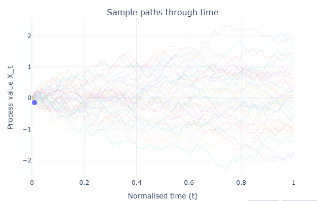
Here is an example of a stochastic process constructed from repeated independent die rolls, whose marginal distributions become approximately Gaussian as time increases. The simulation is based on the following mathematical construction. Let \( D_1, D_2, \dots \) be independent random variables uniformly distributed on \( \{1,…,6 \} \), and define the standardised increments
\( \xi_j = \frac{D_j-\frac72}{\sqrt{35/12}} \).

On the time grid \( t_k=\frac{k}{N}$ for $k = 0,1, \dots, N \) with

$ X_{t_k} = \frac{1}{\sqrt N} \sum_{j=1}^{k}\xi_j $.

Since \( \mathbb{E}[\xi_j = 0 \) and \( \text{Var}(\xi_j) = 1 \), it follows that \( \mathbb E[X_{t_k}]=0 \) and \( \text{Var}(X_{t_k}) = \frac{k}{N} = t_k \). Hence, for sufficiently large \( k \),
\( X_{t_k}\approx\mathcal N(0,t_k). \)
As the number of accumulated increments increases, the marginal distribution of \( X_{t_k} \) becomes approximately Gaussian.

The selected path represents one complete simulated trajectory of the stochastic process, corresponding to a single outcome \( \omega \), while the current value is the point \( X_{t_k}(\omega) \) on that path at the time displayed by the animation. We place the \( N \) discrete steps on the unit time interval by defining \( t_k = k/N \). Thus, \( t_k \) is a dimensionless, normalised time variable representing the proportion of the simulation horizon that has elapsed. In the left-hand panel, the line shows the selected path as it evolves through time and the marker identifies its current position. In the right-hand panel, the same current value is shown relative to the empirical distribution generated from all simulated paths and the accompanying Gaussian approximation, allowing us to compare one realised outcome with the distribution of possible outcomes at that fixed time.

In the next post we'll discuss some important properties of stochastic processes.