The mathematics of Black–Scholes, and why it is not predictive
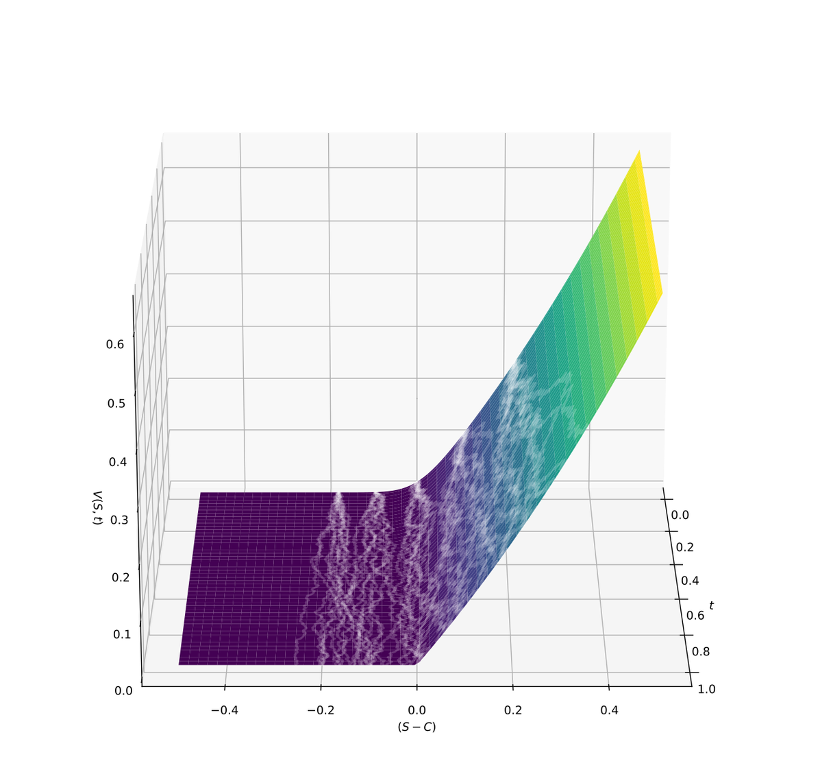
There is a certain elegance to the Black–Scholes equation. From a particular vantage, it looks like physics. It has a diffusion term, a drift term, a boundary condition, and a solution that appears to give randomness structure. For anyone with a physics background and familiarity with stochastic processes, statistical mechanics, or partial differential equations (PDEs), there is an immediate resemblance to heat flow and Brownian motion. This appearance is not superficial. The Black–Scholes equation is a linear parabolic PDE which, under a suitable change of variables, can be transformed into the heat equation. In that sense, the time-decay and diffusion characteristics of option pricing under Black–Scholes can be made to resemble the spread of heat through a medium.
And yet this familiarity can be misleading.
In a number of places on YouTube and in retail trading forums, I have seen Black–Scholes discussed in the context of asset returns as if it were a pricing equation with a statistical prophecy. In practice, Black–Scholes is not a predictive model of realised asset returns, and its analogy with the physical modelling of heat flow can only be taken so far. Although it is equivalent under transformation to the heat equation, the interpretation is very different. The probabilities, volatility input, and stochastic process are not immutable physical constants; they are modelling choices and market-implied quantities. In options pricing, the central role of Black-Scholes is not to forecast where the underlying will go given some set of physical constants. Rather, the goal is to price a hedgeable payoff under idealised no-arbitrage assumptions.
For this reason, and for others that we will discuss, Black–Scholes at best implies a conditional distribution within the model. It contains distributional structure, but that structure depends on variables and assumptions that must be specified or inferred. One could therefore describe it as a model of relative value under idealised trading conditions. It offers a theoretical price for what an option should be worth if the underlying follows a particular stochastic process and if markets are frictionless, trading can occur continuously, volatility is known and constant, borrowing and lending occur at the risk-free rate, and the option payoff can be dynamically hedged. Some of these assumptions are noticeably unrealistic.
What Black–Scholes does not do is tell us where the underlying asset will go, or prove that future prices will politely arrange themselves into a lognormal distribution. It does not estimate the expected return of the stock, determine that markets are Gaussian, or establish that volatility is truly constant.
The stochastic assumption
The model begins by assuming that the underlying asset price follows geometric Brownian motion:
\[ dS_t = \mu S_t dt + \sigma S_t dW_t. \]
Here \( (S_t) \) is the asset price, \( \mu \) is the drift, \( \sigma \) is volatility, and \( W_t \) is a standard Brownian motion.
This is a strong modelling assumption. The asset price is assumed to have continuous paths, proportional volatility, and normally distributed log returns over finite intervals. More precisely, applying Itô’s lemma (I will discuss Itô’s lemma in a future entry) to \( \log S_t \) gives
\[ d \log S_t = \left(\mu - \frac{1}{2}\sigma^2\right)dt + \sigma dW_t. \]
Integrating from \( 0 \) to \( T \), we obtain
\[ \log S_T = \log S_0 + \left(\mu - \frac{1}{2}\sigma^2\right)T + \sigma W_T, \]
so that \( S_T \) is lognormally distributed under the assumed physical dynamics. This is the point at which it is tempting to say: the model predicts a distribution for future prices. But the central mathematical move in Black–Scholes is that this physical drift \( \mu \) disappears from the option-pricing equation. That disappearance is not a minor technical feature; it is, in fact, the essence of the model.
The option as a function of the underlying
Why does the drift disappear in Black-Scholes? Intuitively, one might think if a stock has higher drift, this should correlate with a higher probability of finishing in-the-money (and higher probability of having higher payoff).
Let's explore the drift \( \mu \) more closely. To do that, we will first derive Black-Scholes as a function of the underlying.
Let \( V(S,t) \) denote the price of a derivative written on \( S \). We assume \( V \) is sufficiently smooth in \( S \) and \( t \), and we apply Itô’s lemma:
\[ dV = \frac{\partial V}{\partial t}dt + \frac{\partial V}{\partial S}dS + \frac{1}{2}\frac{\partial^2 V}{\partial S^2}(dS)^2. \]
Since
\[ dS = \mu S dt + \sigma S dW, \]
and since \( (dW)^2 = dt \) in the Itô calculus, this becomes
\[ dV = \left( \frac{\partial V}{\partial t} + \mu S \frac{\partial V}{\partial S} + \frac{1}{2}\sigma^2 S^2 \frac{\partial^2 V}{\partial S^2} \right)dt + \sigma S \frac{\partial V}{\partial S}dW. \]
This stochastic differential expression is the foundation for deriving the Black-Scholes-Merton equation, when coupled with delta-hedging principles and no-arbitrage arguments. Indeed, inspect the above and notice the derivative inherits randomness from the underlying. The stochastic term is proportional to
\[ \sigma S \frac{\partial V}{\partial S}, \]
which is the option’s local exposure to the Brownian shock in the underlying. In trading language, the coefficient \(\partial V/\partial S \) is the option’s delta.
The key insight is that we can form a portfolio that eliminates this local randomness. To understand what this means, let's consider a simple example. Consider a portfolio
\[ \Pi = V - \Delta S, \]
where we choose
\[ \Delta = \frac{\partial V}{\partial S}. \]
The differential of the portfolio is
\[ d\Pi = dV - \Delta dS, \]
assuming a self-financing and dynamically rebalanced portfolio.
Substituting the expressions for \( dV \) and \( dS \), and setting \( \Delta = \partial V/\partial S \), the stochastic \( dW \) terms cancel. The portfolio becomes locally riskless:
\[ d\Pi = \left( \frac{\partial V}{\partial t} + \frac{1}{2}\sigma^2 S^2 \frac{\partial^2 V}{\partial S^2} \right)dt, \]
with vanishing drift \( \mu \) as anticipated. We see that the expected return of the stock is no longer part of the pricing equation because the construction is not trying to forecast the stock’s return. It is constructing a local hedge that neutralises exposure to the stock’s instantaneous randomness.
In other words, if the portfolio is locally riskless, then under the no-arbitrage assumption it must earn the risk-free rate. Since
\[ \Pi = V - S\frac{\partial V}{\partial S}, \]
we require
\[ d\Pi = r\Pi dt. \]
Therefore,
\[ \frac{\partial V}{\partial t} + \frac{1}{2}\sigma^2 S^2 \frac{\partial^2 V}{\partial S^2} = r\left( V - S\frac{\partial V}{\partial S} \right). \]
Simple rearranging gives the Black–Scholes partial differential equation
\[ \frac{\partial V}{\partial t} + \frac{1}{2}\sigma^2 S^2 \frac{\partial^2 V}{\partial S^2} + rS\frac{\partial V}{\partial S} - rV = 0 \]
as the mathematical description of risk-neutral pricing.
The risk-neutral measure
There is another way to express the same result. Under the physical measure, often denoted \( \mathbb{P} \), the underlying follows
\[ dS_t = \mu S_t dt + \sigma S_t dW_t^{\mathbb{P}}. \]
Under the risk-neutral measure, denoted \(\mathbb{Q} \), the drift becomes the risk-free rate
\[ dS_t = r S_t dt + \sigma S_t dW_t^{\mathbb{Q}}, \]
assuming a non-dividend paying stock with a constant risk-free rate. More generally, in practical derivatives pricing one would write
\[ dS_t = (r-q)S_t dt + \sigma S_t dW_t^{\mathbb{Q}} \]
with \( q \) the continuous dividend yield. Keeping \( q = 0 \), the derivative price is written as the discounted expectation of its payoff under \(\mathbb{Q} \):
\[ V(S,t) = e^{-r(T-t)} \mathbb{E}^{\mathbb{Q}} \left[ \Phi(S_T)\mid S_t=S \right], \]
where \(\Phi(S_T) \) is the terminal payoff.
For a European call,
\[ \Phi(S_T) = \max(S_T-K,0), \]
the famous formula is
\[ C = S_0 N(d_1) - K e^{-rT}N(d_2), \]
with
\[ d_1 = \frac{ \ln(S_0/K) + \left(r+\frac{1}{2}\sigma^2\right)T}{\sigma\sqrt{T}}, \]
and
\[ d_2 = d_1 - \sigma\sqrt{T}. \]
This formula is often presented as though it were a probabilistic forecast. In a naive way, it is an understandable interpretation; because it contains a cumulative normal distribution \( N(\cdot) \), and because the derivation involves a distribution for \( S_T \). But the expectation here is not an expectation under the real-world probability measure. It is an expectation under the risk-neutral measure. This distinction is not simply philosophical, it is deeply quantitative and of direct mathematical consequence.
So, what have we learned? The risk-neutral measure is a pricing measure. It is the probability measure under which discounted tradable asset prices are martingales (as per the description of this type of PDE via the Feynman–Kac formula). More technically, in a complete no-arbitrage market, the risk-neutral measure is the equivalent martingale measure under which discounted tradable asset prices are martingales. In the Black–Scholes setting, market completeness makes this measure unique, which is why the derivative has a unique replication price. It is not, however, the measure that describes the empirical frequency with which markets move.
In other words, \( \mathbb{Q} \) is not \( \mathbb{P} \).
The Black–Scholes formula prices the option by evaluating the payoff under \( \mathbb{Q} \), not by predicting the realised path under \( \mathbb{P} \). (The latter will be the topic of a future post, where we will want to quantitatively describe realised paths and their statistical ensemble).
For now, though, we can conclude by noting that the disappearance of \( \mu \) is an important conceptual result in quantitative finance. Although the drift disappears, volatility remains. If one were valuing the option by taking a real-world expected payoff under \( \mathbb{P} \), then the expected return of the underlying would matter. But Black–Scholes does not price the option that way. It prices the option by replication. If one were valuing the option by subjective expected payoff, an investor who expects a stock to rise by 20% would value a call differently from an investor who expects it to fall by 20%. But in the idealised Black-Scholes world, the no-arbitrage price does not depend on subjective expected return. It depends on the current stock price, strike, time to expiry, risk-free rate, and volatility. This is because the option is priced by replication, not by belief. If the option payoff can be replicated through continuous trading in the stock and cash account, then the cost of that replicating strategy determines the option price. If the option traded above that cost, one could sell the option and buy the replicating portfolio. If it traded below that cost, one could buy the option and sell the replicating portfolio. In either case, arbitrage would force consistency.